Metrics
📈 Introduction
What are they for?
They provide context of what happened and the trend
- Numerical data over time: CPU, latency, number of requests
- Key to alerting and SLA/SLO
- Low-cost and efficient
Tools: Prometheus, Grafana Mimir, InfluxDB
🎯 Use of Metrics vs. Metrics in Logs
📊 Why dedicated metrics systems?
Metrics are numerical time-series data optimized for:
- Fast aggregations (sum, average, percentiles)
- Efficient storage (compression, downsampling)
- Lightning-fast queries (time-based indexing)
- Real-time alerting
⚡ The problem with metrics in logs
❌ Bad approach - metrics as logs:
{"timestamp": "2025-10-27T10:00:00Z", "level": "info", "message": "Request processed", "response_time": 250, "status": 200}
{"timestamp": "2025-10-27T10:00:01Z", "level": "info", "message": "Request processed", "response_time": 180, "status": 200}
{"timestamp": "2025-10-27T10:00:02Z", "level": "info", "message": "Request processed", "response_time": 420, "status": 500}
✅ Good approach - dedicated metrics:
# Prometheus format
http_request_duration_seconds{method="GET",status="200"} 0.250
http_request_duration_seconds{method="GET",status="200"} 0.180
http_request_duration_seconds{method="GET",status="500"} 0.420
💾 Storage Comparison
Scenario: 1000 requests/second for 1 hour
📋 Metrics in logs (JSON):
{"ts":"2025-10-27T10:00:00Z","msg":"Request","duration":250,"status":200,"method":"GET","endpoint":"/api/users"}
- Single entry size: ~110 bytes
- 1000 req/s × 3600s × 110B = 396 MB/hour
- 396 MB × 24h = 9.5 GB/day
📊 Dedicated metrics (Prometheus):
http_request_duration_seconds{method="GET",endpoint="/api/users",status="200"} 0.250 1698412800
- Single entry size: ~85 bytes
- But with time compression: 1000 points → ~15 points/minute (aggregation)
- 15 × 60 minutes × 85B = 76.5 KB/hour
- 76.5 KB × 24h = 1.8 MB/day
📈 Efficiency Difference
| Aspect | Metrics in logs | Dedicated metrics | Improvement |
|---|---|---|---|
| Disk space | 9.5 GB/day | 1.8 MB/day | 5277x less! |
| Query time | 5-10 seconds | 50-100ms | 50-100x faster |
⚖️ When to use logs vs metrics?
| Data | Logs | Metrics | Reason |
|---|---|---|---|
| Application errors | ✅ | ❌ | Context and stack trace needed |
| Response times | ❌ | ✅ | Aggregations, percentiles, alerting |
| Request count | ❌ | ✅ | Sums, trends, dashboards |
| Business events | ✅ | ✅ | Logs for context, metrics for KPIs |
| User actions | ✅ | ❌ | Detailed behavior tracking |
| System resources | ❌ | ✅ | Monitoring, alerting, autoscaling |
📊 Metric Types
🔢 1. Counter
![]()
Definition: A value that only increases (or resets to zero)
Examples:
http_requests_total{method="GET", status="200"} 1547
errors_total{service="payment"} 23
bytes_sent_total{endpoint="/api/users"} 2048576
Characteristics:
- ✅ Monotonic (always goes up)
- ✅ Ideal for counting events
- ✅ Can calculate rate (increase per second)
- ❌ Does not show current value
Use cases:
- Number of HTTP requests
- Number of errors
- Number of processed tasks
- Bytes sent over network
PromQL examples:
# Rate - requests per second
rate(http_requests_total[5m])

# Increase in the last 5 minutes
increase(http_requests_total[5m])
📏 2. Gauge
![]() Definition: A value that can increase and decrease - shows current state
Definition: A value that can increase and decrease - shows current state
Examples:
cpu_usage_percent{host="web01"} 85.2
memory_available_bytes{host="web01"} 2147483648
active_connections{service="database"} 42
queue_size{queue="orders"} 156
Characteristics:
- ✅ Can increase and decrease
- ✅ Shows current value
- ✅ Ideal for alerting
- ❌ Historical trend is not inherently meaningful per se
Use cases:
- CPU/RAM usage
- Temperature
- Number of active connections
- Queue size
- Number of active users
PromQL examples:
# Average CPU usage in the last 5 minutes
avg_over_time(cpu_usage_percent[5m])

# Maximum memory usage
max_over_time(memory_usage_percent[1h])
📈 3. Histogram
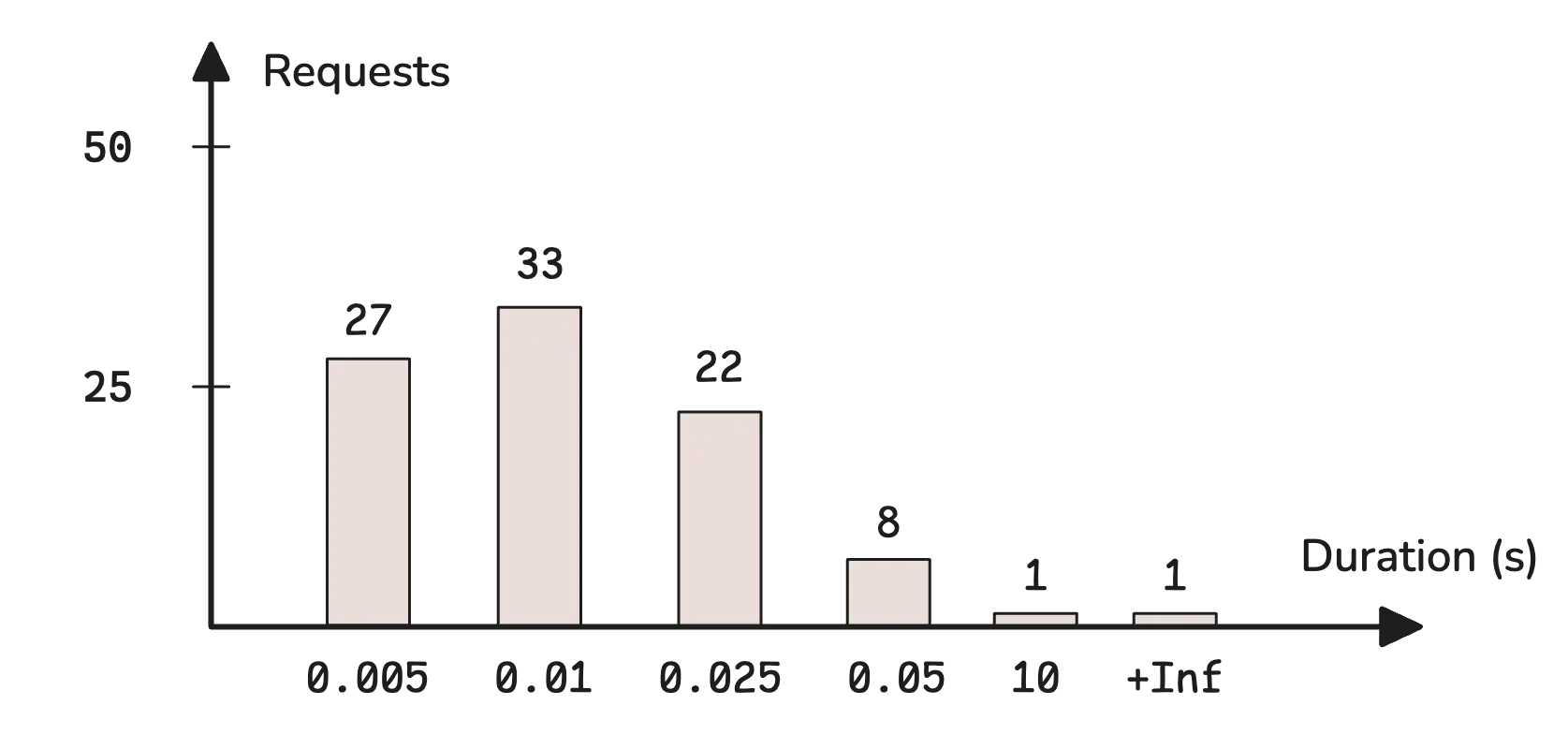
Definition: Counts observations in predefined buckets (ranges)
Example structure:
http_request_duration_seconds_bucket{le="0.1"} 2450
http_request_duration_seconds_bucket{le="0.5"} 4321
http_request_duration_seconds_bucket{le="1.0"} 4890
http_request_duration_seconds_bucket{le="2.0"} 4950
http_request_duration_seconds_bucket{le="+Inf"} 5000
http_request_duration_seconds_sum 2847.3
http_request_duration_seconds_count 5000
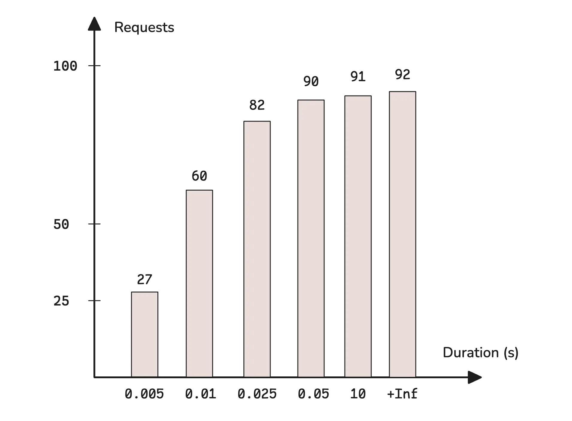
What you get:
- Buckets - number of observations in each range
- Sum - sum of all values
- Count - total number of observations
Use cases:
- Response time
- Request size
- Processing duration
- SLA/percentile monitoring
PromQL examples:
# 95th percentile response time
histogram_quantile(0.95, rate(http_request_duration_seconds_bucket[5m]))

# Average response time
rate(http_request_duration_seconds_sum[5m]) / rate(http_request_duration_seconds_count[5m])

# Percentage of requests below 500ms
rate(http_request_duration_seconds_bucket{le="0.5"}[5m]) / rate(http_request_duration_seconds_count[5m])
📈 3a. Native Histogram
Definition: Native histograms (also known as sparse histograms) are a new generation of histograms in Prometheus (since v2.40) that automatically select buckets based on observed values, eliminating the need for manual configuration.
Key differences vs classic histogram:
| Aspect | Classic Histogram | Native Histogram |
|---|---|---|
| Buckets | Manually predefined | Automatic (exponential) |
| Time series | One per bucket (le=”…”) | One series per metric |
| Data size | Grows with number of buckets | Constant, compact |
| Accuracy | Depends on bucket selection | Controlled by resolution schema |
| Configuration | Requires choosing boundaries | Minimal — works out-of-the-box |
How it works:
- Buckets based on powers of 2 (exponential boundaries)
- Schema parameter (from -4 to 8) controls resolution — higher schema = more buckets = greater accuracy
- Stored as a single time series instead of multiple
_bucketseries
Internal JSON structure:
A native histogram sample is stored as a single structured object:
{
  "schema": 3,
  "count": 1500,
  "sum": 87.3,
  "zero_threshold": 0.001,
  "zero_count": 12,
  "positive_spans": [
    { "offset": 0, "length": 3 },
    { "offset": 2, "length": 2 }
  ],
  "positive_deltas": [45, -12, 8, 30, -5],
  "negative_spans": [
    { "offset": 1, "length": 2 }
  ],
  "negative_deltas": [10, 3]
}
| Field | Description |
|---|---|
schema |
Bucket resolution (-4 to 8). Higher = more buckets, finer accuracy |
count |
Total number of observations |
sum |
Sum of all observed values |
zero_threshold |
Half-width of the zero bucket — observations in [-threshold, +threshold] go here |
zero_count |
Number of observations in the zero bucket |
positive_spans |
Describes which positive buckets are populated. Each span has an offset (gap from previous) and length (consecutive populated buckets) |
positive_deltas |
Delta-encoded counts for populated positive buckets |
negative_spans / negative_deltas |
Same as above, for negative observed values |
Decoding the example above (schema 3):
With schema 3, there are 8 buckets per power of 2. Bucket boundaries: boundary(i) = 2^(i/8)
positive_spans: [{offset:0, length:3}, {offset:2, length:2}] means:
- First span starts at bucket index 0, covers 3 consecutive buckets (indices 0, 1, 2)
- Second span skips 2 empty buckets (indices 3, 4), covers 2 buckets (indices 5, 6)
positive_deltas: [45, -12, 8, 30, -5] — delta-encoded, each value adds to the previous count:
Bucket  Boundaries (schema 3)      Delta   Count (cumulative delta)
──────  ─────────────────────────   ─────   ────────────────────────
  0     [1.000,  1.091)              +45     45
  1     [1.091,  1.189)              -12     33
  2     [1.189,  1.297)               +8     41
  3     [1.297,  1.414)             (empty — skipped by span offset)
  4     [1.414,  1.542)             (empty — skipped by span offset)
  5     [1.542,  1.682)              +30     71
  6     [1.682,  1.834)               -5     66
negative_spans: [{offset:1, length:2}] / negative_deltas: [10, 3] — same logic, mirrored:
Bucket  Boundaries (schema 3)      Delta   Count
──────  ─────────────────────────   ─────   ─────
  0     [-1.091, -1.000)            (empty — skipped by offset 1)
  1     [-1.189, -1.091)             +10     10
  2     [-1.297, -1.189)              +3     13
zero_count: 12 — 12 observations fell in the zero bucket [-0.001, +0.001]

Schema parameter and bucket growth:
The schema controls how many buckets exist per power of 2. Bucket boundaries follow the formula: boundary(i) = 2^(i * 2^(-schema))
| Schema | Growth factor | Buckets per power of 2 | Bucket boundaries (starting at 1) | Use case |
|---|---|---|---|---|
| -4 | ~65536 | 1/16 | 1, 65536, … | Extremely coarse — huge-range counters |
| 0 | 2 | 1 | 1, 2, 4, 8, 16, 32, … | Coarse — order-of-magnitude grouping |
| 1 | ~1.41 | 2 | 1, 1.41, 2, 2.83, 4, … | Low resolution |
| 2 | ~1.19 | 4 | 1, 1.19, 1.41, 1.68, 2, … | Moderate |
| 3 | ~1.09 | 8 | 1, 1.09, 1.19, 1.30, 1.41, … | Default — good balance |
| 5 | ~1.02 | 32 | 1, 1.02, 1.04, 1.06, … | High precision |
| 8 | ~1.003 | 256 | 1, 1.003, 1.005, … | Maximum precision — microsecond latency |
Higher schema = exponentially more buckets = better percentile accuracy, but more memory. Schema 3 (default) gives ~6.7% relative error on quantile estimation — sufficient for most use cases.
Example — classic vs native:
# Classic histogram: 5+ time series
http_request_duration_seconds_bucket{le="0.1"} 2450
http_request_duration_seconds_bucket{le="0.5"} 4321
http_request_duration_seconds_bucket{le="1.0"} 4890
http_request_duration_seconds_bucket{le="+Inf"} 5000
http_request_duration_seconds_sum 2847.3
http_request_duration_seconds_count 5000

# Native histogram: 1 time series contains all buckets!
http_request_duration_seconds  →  {schema:5, count:5000, sum:2847.3,
                                    positive_spans:[...], positive_deltas:[...]}
Example — Go instrumentation:
import (
    "github.com/prometheus/client_golang/prometheus"
    "github.com/prometheus/client_golang/prometheus/promauto"
)

requestDuration := promauto.NewHistogram(prometheus.HistogramOpts{
    Name: "http_request_duration_seconds",
    Help: "Duration of HTTP requests.",
    // Native histogram configuration:
    NativeHistogramBucketFactor:     1.1,  // ~schema 3
    NativeHistogramMaxBucketNumber:  100,  // limit memory usage
    NativeHistogramZeroThreshold:    0.001,
})

// Usage — identical to classic histogram:
requestDuration.Observe(0.235)
Enabling in Prometheus:
# prometheus.yml - global enablement
global:
  scrape_protocols:
    - PrometheusProto        # required for native histograms
    - OpenMetricsText1.0.0
    - OpenMetricsText0.0.1
    - PrometheusText1.0.0
    - PrometheusText0.0.4

# Enable feature flag when starting Prometheus:
# --enable-feature=native-histograms
PromQL — queries work the same:
# 95th percentile — identical syntax as for classic histogram
histogram_quantile(0.95, rate(http_request_duration_seconds[5m]))

# Average response time
rate(http_request_duration_seconds_sum[5m]) / rate(http_request_duration_seconds_count[5m])
When to use Native Histogram:
- ✅ Prometheus >= 2.40 and you want to reduce cardinality (fewer time series)
- ✅ You don’t know what buckets to choose — native histogram adapts automatically
- ✅ You need more accurate percentiles without increasing the number of buckets
- ✅ You have many histogram metrics and want to save storage/memory
- ❌ Not yet supported by all tools (e.g., older versions of Grafana, Thanos)
💡 Tip: You can configure dual scraping — Prometheus collects both classic and native histograms simultaneously, making migration easier.
📐 4. Summary
![]()
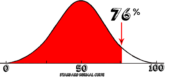
Definition: Similar to histogram, but with pre-calculated quantiles
Example structure:
http_request_duration_seconds{quantile="0.5"} 0.235
http_request_duration_seconds{quantile="0.9"} 0.821
http_request_duration_seconds{quantile="0.95"} 1.234
http_request_duration_seconds{quantile="0.99"} 2.156
http_request_duration_seconds_sum 2847.3
http_request_duration_seconds_count 5000
Characteristics:
- ✅ Pre-calculated quantiles (fast queries)
- ✅ Accurate percentile values
- ❌ Cannot aggregate across instances
- ❌ Quantiles fixed at application level
Use cases:
- Response time (when you need accurate percentiles)
- Processing time
- Queue wait time
⚖️ Histogram vs Summary
| Aspect | Histogram | Summary |
|---|---|---|
| Percentiles | Approximated | Exact |
| Aggregation | ✅ Possible across instances | ❌ Not possible |
| Overhead | Lower | Higher |
| Flexibility | ✅ Quantiles in PromQL | ❌ Fixed upfront |
| Usage | Recommended for most cases | When you need exact percentiles |
🎨 Metric Naming Best Practices
Two similar standards:
Conventions
# Counter - ends with _total
http_requests_total
errors_total
bytes_sent_total

# Gauge - describes current state
cpu_usage_percent
memory_available_bytes
active_connections

# Histogram/Summary - ends with unit + _bucket/_sum/_count
response_time_seconds_bucket
request_size_bytes_bucket

# Base units (SI)
_seconds (not _milliseconds)
_bytes (not _kilobytes)
_total (for counters)
Labels
# Good
http_requests_total{method="GET", status="200", endpoint="/api/user"}

# Bad - too high cardinality
http_requests_total{user_id="123456", session="abc-def-ghi"}
🛠️ Practical Tips
✅ DO:
- Use metrics for everything that can be counted, measured, aggregated
- Log context, errors, unusual events
- Implement metrics at both application and infrastructure level
- Set alerts on metrics, not on logs
❌ DON’T:
- Don’t log numerical data that repeats regularly
- Don’t use logs for performance monitoring
- Avoid real-time alerting on logs
- Don’t mix business metrics with diagnostic logs
Handling Infrequent Metrics
Some metrics are reported very rarely — for example, once every 6 hours (batch job results, daily aggregations, periodic health checks). This creates specific challenges in both Prometheus and OpenTelemetry.
The Problems
1. rate() / increase() return empty results
These functions need at least 2 samples within the query window. If a metric arrives every 6 hours but the query range is [5m], there is nothing to compute.
Fix: set the query window to at least 2× the reporting interval:
rate(batch_job_records_total[13h])      # 2 × 6h + margin
increase(batch_job_records_total[13h])
2. Staleness — series disappear after ~5 minutes
In the pull model, Prometheus marks a series as stale if no new sample arrives within ~5 minutes of the last scrape. After that, instant queries return no data.
Workarounds:
- Use range queries instead of instant queries
- Use
last_over_time()to surface the most recent value:last_over_time(batch_job_status[7h]) - In Grafana, set the query range /
$__rate_intervalto match the reporting frequency
OTel Push Model — the natural solution
With OpenTelemetry, the application pushes metrics via OTLP. This avoids the pull-model staleness problem entirely:
App (OTel SDK) → OTLP push → OTel Collector → remote write → Prometheus / Mimir
Why this helps:
- No staleness from missed scrapes — the metric arrives with its original timestamp via remote write
- The Collector handles batching, retry, and queuing — the app fires and forgets
- No extra components needed — if you already use OTel, the pipeline is already there
Pushgateway is redundant with OTel
If the application already uses the OTel SDK, adding a Pushgateway adds complexity without value:
| Pushgateway | OTel Collector | |
|---|---|---|
| Protocol | Custom HTTP PUT | OTLP (standard) |
| TTL / cleanup | None (manual delete) | Not needed (flow-through) |
| Retry / queue | None | Built-in |
| Multi-backend | No | Yes (Prometheus, Mimir, Tempo, Loki…) |
Rule of thumb: If the app has the OTel SDK → use the OTLP push path. Reserve Pushgateway only for legacy scripts that cannot be instrumented with OTel.
Collector configuration for infrequent metrics
receivers:
  otlp:
    protocols:
      grpc:
        endpoint: 0.0.0.0:4317

exporters:
  prometheusremotewrite:
    endpoint: "http://mimir:9009/api/v1/push"

service:
  pipelines:
    metrics:
      receivers: [otlp]
      exporters: [prometheusremotewrite]
Query window cheat sheet
| Reporting interval | Minimum query window | Example |
|---|---|---|
| 1 hour | [2h30m] |
rate(x[2h30m]) |
| 6 hours | [13h] |
increase(x[13h]) |
| 24 hours | [49h] |
last_over_time(x[49h]) |
Key rule: the query window must be at least 2× the reporting interval — otherwise
rate(),increase(), andavg_over_time()will produce gaps or zeros.
Formats
🎯 Prometheus - Exposition Format
Format:
# HELP metric_name Description of the metric
# TYPE metric_name metric_type
metric_name{label1="value1",label2="value2"} metric_value timestamp
Example:
# HELP cpu_usage_percent Current CPU usage percentage
# TYPE cpu_usage_percent gauge
cpu_usage_percent{host="server01",region="us-west",service="web-app"} 85.2 1698412800000

# HELP http_requests_total Total number of HTTP requests
# TYPE http_requests_total counter
http_requests_total{method="GET",status="200",endpoint="/api/users"} 1500 1698412800000

# HELP memory_usage_bytes Memory usage in bytes
# TYPE memory_usage_bytes gauge
memory_usage_bytes{host="server01",region="us-west",type="available"} 2048000000 1698412800000
memory_usage_bytes{host="server01",region="us-west",type="used"} 6144000000 1698412800000
Prometheus Structure:
- Metric Name - metric name (e.g.,
cpu_usage_percent) - Labels - key-value pairs in
{}(e.g.,{host="server01"}) - Value - single numerical value
- Timestamp - Unix timestamp in milliseconds (optional)
Prometheus Advantages:
- ✅ Wide ecosystem and adoption (CNCF)
- ✅ Built-in alerting (Alertmanager)
- ✅ Pull model - better for service discovery
- ✅ PromQL - powerful query language
- ✅ Federation and hierarchical deployment
Prometheus Disadvantages:
- ❌ One value per metric (requires multiple metrics for complex data types)
- ❌ Limited long-term retention capabilities
- ❌ Issues with high label cardinality
🌐 OpenTelemetry - OTLP Metrics Format
Format (JSON):
{
  "resourceMetrics": [{
    "resource": {
      "attributes": [{
        "key": "service.name",
        "value": {"stringValue": "web-app"}
      }]
    },
    "scopeMetrics": [{
      "metrics": [{
        "name": "http_request_duration",
        "unit": "s",
        "gauge": {
          "dataPoints": [{
            "timeUnixNano": "1698412800000000000",
            "asDouble": 0.250,
            "attributes": [{
              "key": "method",
              "value": {"stringValue": "GET"}
            }]
          }]
        }
      }]
    }]
  }]
}
Format (Protobuf - binary):
message ResourceMetrics {
  Resource resource = 1;
  repeated ScopeMetrics scope_metrics = 2;
}
Practical example (JSON):
{
  "resourceMetrics": [{
    "resource": {
      "attributes": [
        {"key": "service.name", "value": {"stringValue": "payment-service"}},
        {"key": "service.version", "value": {"stringValue": "1.2.3"}},
        {"key": "host.name", "value": {"stringValue": "server01"}}
      ]
    },
    "scopeMetrics": [{
      "scope": {
        "name": "payment-instrumentation",
        "version": "0.1.0"
      },
      "metrics": [
        {
          "name": "http_requests_total",
          "description": "Total HTTP requests",
          "unit": "1",
          "sum": {
            "aggregationTemporality": 2,
            "isMonotonic": true,
            "dataPoints": [{
              "timeUnixNano": "1698412800000000000",
              "asInt": "1500",
              "attributes": [ /*Labels*/
                {"key": "method", "value": {"stringValue": "GET"}},
                {"key": "status_code", "value": {"intValue": "200"}}
              ]
            }]
          }
        },
        {
          "name": "response_time_histogram",
          "description": "HTTP response time distribution",
          "unit": "s", /*Unit*/
          "histogram": { /*Type*/
            "aggregationTemporality": 2,
            "dataPoints": [{
              "timeUnixNano": "1698412800000000000",
              "count": "100",
              "sum": 25.0,
              "bucketCounts": ["10", "30", "40", "20"],
              "explicitBounds": [0.1, 0.5, 1.0, 2.0]
            }]
          }
        }
      ]
    }]
  }]
}
OpenTelemetry Structure:
- Resource - resource metadata (service.name, host.name)
- Scope - instrumentation scope (library, version)
- Metrics - list of metrics with data
- DataPoints - data points with timestamps and attributes
OpenTelemetry Metric Types:
- Gauge - current value (like Prometheus gauge)
- Sum - cumulative sum (like Prometheus counter)
- Histogram - value distribution in buckets
- ExponentialHistogram - histogram with exponential buckets (Native histogram)
OpenTelemetry Advantages:
- ✅ Vendor-neutral - works with many backends
- ✅ Standardization across traces, logs, and metrics
- ✅ Rich data model (Resource + Scope + Attributes)
- ✅ Support for both push and pull
- ✅ Automatic instrumentation for many languages
- ✅ Support for sampling and batching
OpenTelemetry Disadvantages:
- ❌ Higher overhead compared to simpler formats
- ❌ Complexity - more layers of abstraction
- ❌ Newer standard - less operational experience
- ❌ Requires OTel Collector for full functionality
This configuration demonstrates the power of OpenTelemetry - one Collector can receive metrics in both OTel and Prometheus formats, and then export them to different backends!